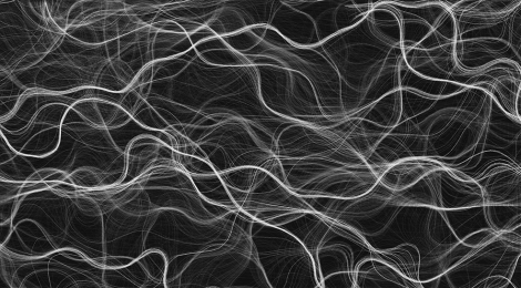
In this post I will write about how I created the following Perlin noise-based visual graphics using the Java programming language.

Code for the original project can be found here: https://github.com/PierpaoloLucarelli/PerlinNoiseVectorField

Video demonstration of the project:

This post is not intended to cover how the Perlin noise algorithm works, but it is simply meant to give the reader an idea on how to create a visualisation like the the one in the above picture.

I did not implement the Perlin noise algorithm myself, but I have used this Java code: http://mrl.nyu.edu/~perlin/noise/

If you are not familiar with the Perlin noise algorithm I recommend this post: https://www.khanacademy.org/computing/computer-programming/programming-natural-simulations/programming-noise/a/perlin-noise

So lets get started with the post 🙂

Step 1 | Creating a vector flow field

The Perlin noise visualisation was created by dropping ‘particles’ on a plane and tracing their path as they move in space. The direction and velocity of these particles is determined by a vector flow field.

To create a vector field, divide a plane into a grid of n by m squares. On each top corner of the square we will place a vector with a chosen magnitude (A good starting point is a magnitude of 1). Settings the angle as a random value would generate pure noise, but that is not what we want. Instead we will se the angle of the vector (x,y) as a Perlin noise value based on the x,y coordinates of the vector itself. This will create something like this:

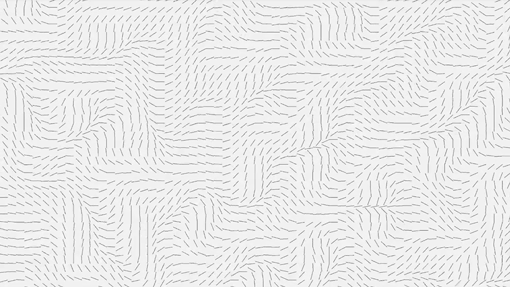
To make the vector field move in time (as seen in the youtube video) we will make pass a third parameter to the Perlin noise algorithm: Time. So the angle of vectors the will be given by:

angle = perlinNoise(x,y,time);

Step 2 | Drop particles on the plane

Next we will place particles in the vector field at a random spot. A particle will be described by 3 vectors:

1. Position
2. Velocity
3. Acceleration

As we said the initial position of the particle will be given by a vector initialised at random x and y coordinates. The position of the particle will change according to it’s velocity. To make the particle move in space we will add the velocity vector to the position vector and to make the velocity change we will add the acceleration to the velocity.

As you maybe guessed the acceleration of the particle will be given by the vector that is currently in under the particle. To figure out what vector the particle is currently over, first we divide the x and y coordinates of the particle by the size of the squares of the grid. This will give us the coordinates of the square under the particle. Then we lookup the vector in that square and add it to the acceleration of the particle.

This will cause the particles to follow the vector field.

We will also need to implement some boundaries check to allow the particles to re-enter the field in the opposite position to where they left the plane.

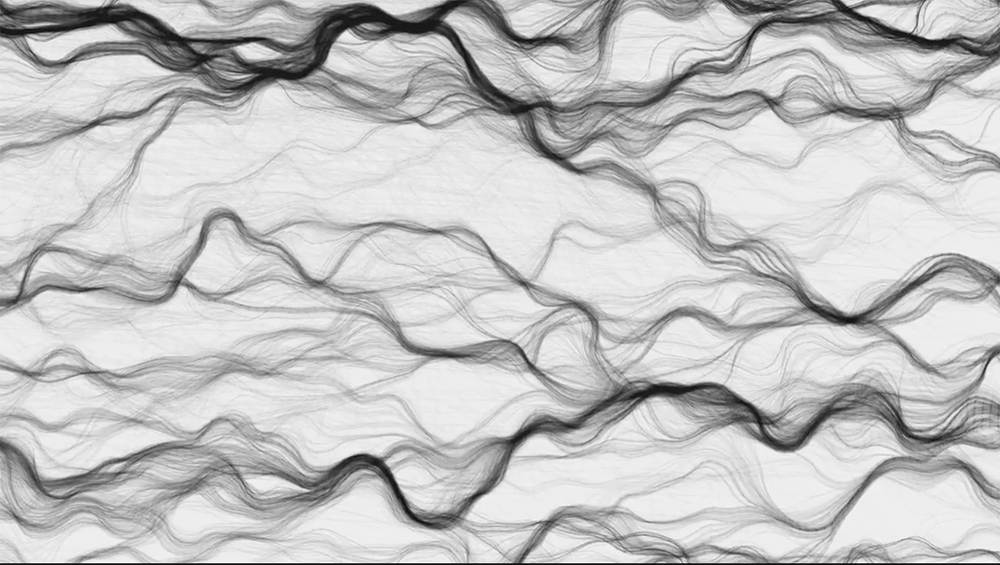
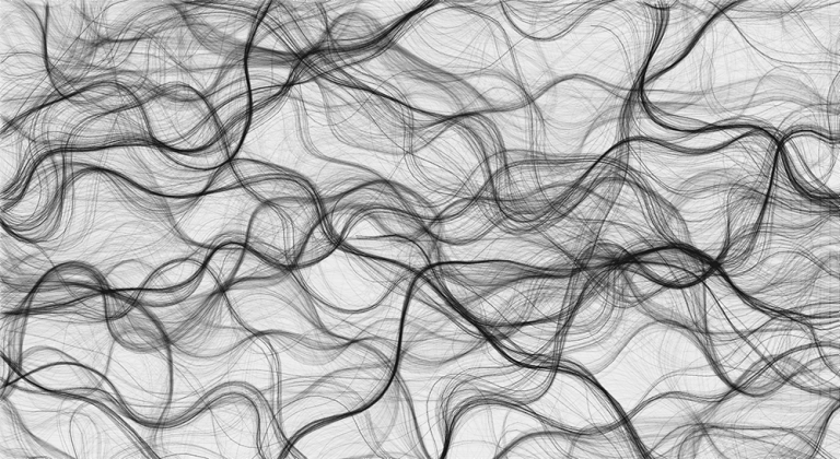
Step 3 | Trace the path of the particles

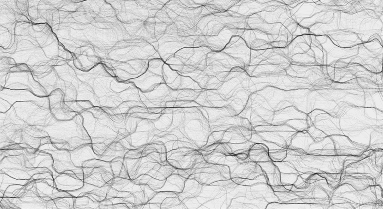
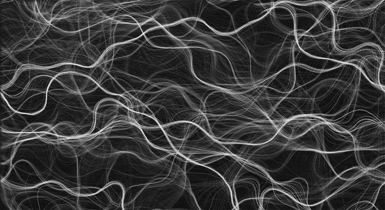
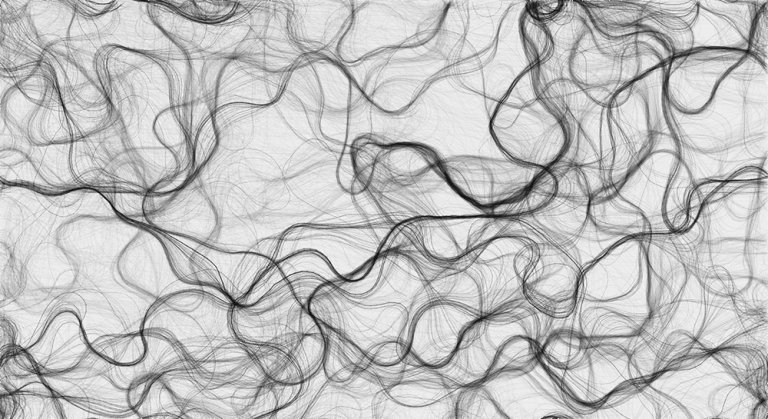
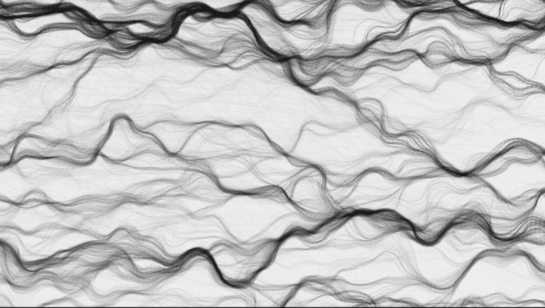
Now the only thing that is left is to trace the path that the particles make over time, and we will be left with awesome Perlin noise visualisation such as these:

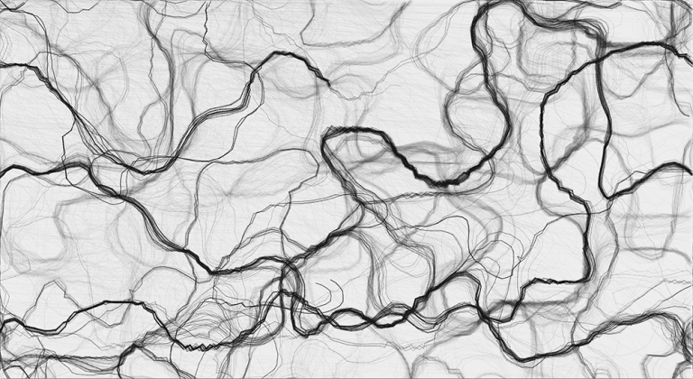
And that’s it 🙂

Some details of the implementation have been left out, but you can look at my code on Github and ask questions in the comment section.